Bi-directional Rapidly-exploring Random Tree (B-RRT) algorithm for a quadrotor moving in 3D-space
Georgios Apostolides, Guru Deep Singh , Kevin Voogd , Markos Gkozntaris
Abstract
This project focuses on the path planning algorithm for a quadrotor - a Bi-directional Rapidly-exploring Random Tree (B-RRT). The algorithm devised optimizes the list of vertices sampled to provide locally optimized planned trajectory. The advantage of B-RRT over traditional RRT is reduced computation time and locally optimized path to goal. We present the algorithm as a simple extension to RRT that could be further extended by more advanced path-planning algorithms. The path computed is smoothened using minimum snap and is then simulated on MATLAB, generating a collision free trajectory while complying with the dynamics of quadrotor.
1. INTRODUCTION
The project presents the modelling of a Crazyflie 2.0 quadrotor developed by Bitcraze, which is controlled using a position and an attitude controller to follow a trajectory computed using Rapidly-exploring Random Trees (RRT) algorithm and its extensions in order to avoid collision with the obstacles present in the given map.
The objective of the project is to plan a path for the quadrotor from a start to a goal position. The map for the project is chosen as a room ablaze with a human stuck inside and the quadrotor should reach the human and provide him with the necessary tools, such as a oxygen mask, or communication instruments like a mobile phone. The project considers the quadrotor moving in a 3D space with an initial position outside the room and goal position near the human. The assumption undertaken is that the fire is considered to be non-progressive, and hence assumed as a static obstacle.
The high dimensionality of the configuration space, the assumption of static obstacles, as well as, the simplicity and robustness of RRT, makes it the best choice compared to algorithms like Probabilistic Roadmap Method (PRM) or motion primitives. The RRT provides a feasible solution if one is found within the constraint of iterations.
Since, RRT provides only a feasible solution and not an optimal, researchers nowadays are working on improved algorithms such as RRT*, which provide the optimal path. However, these algorithms are inefficient as sampling randomly explores the entire map, and for that reason researchers have tried to guide the sampling in a way to reduce the computation time[1-3]. Apart, from this many other methodologies are also being developed and researched into, like path planning using vector fields, which are in-turn improving the accuracy for path planning[4]. This project employs a bi-birectional guided RRT (B-RRT), which is compared to a traditional RRT. The software package auxiliary to the path planning like for control, simulation, trajectory smoothening, etc are adapted from the project by L. Yiren, C. Myles, L. Wudao and Z. Xuanyu.
2. ROBOT MODEL
2.1 Kinematic Model
The workspace is \(W=R^3\), as the quadrotor can displace to all positions in space provided that there are no obstacles at that place. The configuration space is \(C=SE(3)\)[5]. The robot is able to move forward, in a side direction and upwards. In addition to that it can rotate in 3D space using the three Euler angles: Roll \((\phi)\), Pitch \((\theta)\), Yaw \((\psi)\).
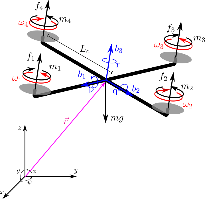
The position and the orientation of the quadrotor in the inertial world frame is \(\mathbf{\xi}_I = [x,y,z,\phi,\theta,\psi]^T\) and the vector containing the linear and angular velocities expressed in the body frame is \(\dot{\mathbf{\xi}}_B = [u,v,w,p,q,r]^T = [\mathbf{v}_B, \mathbf{\omega}_B]^T\). The orthonormal basis vectors that represent the inertial and body-fixed frames are, on the hand hand, \(\mathbf{\hat{a}_1}\), \(\mathbf{\hat{a}_2}\), and \(\mathbf{\hat{a}_3}\), and on the other hand, \(\mathbf{\hat{b}_1}\), \(\mathbf{\hat{b}_2}\), and \(\mathbf{\hat{b}_3}\). In Fig. 1 a schematic drawing is shown, depicting the frames of reference and also the forces and moments acting on the object. The linear velocities in the body-fixed frame are related to the world velocities via a rotation matrix \(\boldsymbol{R}\), and similarly with the angular velocities with a Jacobian matrix \(\boldsymbol{J}\)[6]. In this report, the convention yaw-pitch-roll is used, resulting in the Euler-based rotation matrix \(\mathbf{R}(\phi,\theta,\psi)=R_{z}(\psi)R_{x}(\phi)R_{y}(\theta)\)[7].
\[\textbf{R}=
\begin{pmatrix}
\text{c}\theta \text{c}\psi -\text{s}\phi\text{s}\psi\text{s}\theta & -\text{c}\phi \text{s}\psi & \text{c}\psi\text{s}\theta + \text{c}\theta\text{s}\phi\text{s}\psi\\
\text{c}\theta\text{s}\psi+\text{c}\psi\text{s}\phi\text{s}\theta & \text{c}\phi \text{c}\psi & \text{s}\psi\text{s}\theta - \text{c}\psi\text{c}\theta\text{s}\phi\\
-\text{c}\phi\text{s}\theta & \text{s}\phi & \text{c}\phi \text{c}\theta
\end{pmatrix}\]
where c(\(\cdot\)) and s(\(\cdot\)) are \(\cos({\cdot})\) and \(\sin({\cdot})\) respectively and the angular velocities are related by the inverse Jacobian matrix[8]:
\[\begin{pmatrix}
p \\
q \\
r \\
\end{pmatrix} =
\begin{pmatrix}
\text{c}\theta & 0 & -\text{c}\phi\text{s}\theta\\
0 & 1 & \text{s}\phi \\
\text{s}\theta & 0 & \text{c}\phi\text{c}\theta
\end{pmatrix}
\begin{pmatrix}
\dot{\phi}\\
\dot{\theta}\\
\dot{\psi}
\end{pmatrix}\]
2.2 Dynamic Model
In the dynamic modelling of the quadrotor it is assumed that the only forces acting on it are its own weight and the thrust force. Other forces such as drag are neglected. Then, Newton's second law is derived as:
\[m(\mathbf{\omega}_B\times\mathbf{v}_B+\dot{\mathbf{v}}_B) = \mathbf{F}_B = (f_1+f_2+f_3+f_4)\mathbf{b_3}-mg\mathbf{R}^T\mathbf{a}_3\]
\[\mathbf{I\omega}_B + \mathbf{\omega}_B\times(\mathbf{I\omega}_B) = \mathbf{M}_B = (f_2 - f_4)L_c\mathbf{b_1} + (f_3 - f_1)L_c\mathbf{b_2} + (-m_1+m_2-m_3+m_4)\mathbf{b_3}\]
where \(m\) is the mass of the quadrotor and \(\mathbf{F}_B\) is the resultant force acting on the quadrotor with respect to the body frame. In the second equation, \(\mathbf{I}\) is the diagonal inertia matrix with components \(I_x\), \(I_y\) and \(I_z\) and \(\mathbf{M}_B\) is the resultant moment expressed in body-frame coordinates. The forces and the moments are related to the speed of the motors as \(f_i = k_F\omega_i^2\) and \(m_i = k_M\omega_i^2\), where \(k_F\) and \(k_M\) are constants and \(\omega_i\) is the angular speed of the rotor. The ratio of these two constants is expressed as \(\gamma = \frac{k_M}{k_F}\).
2.3 Linearization
The system is linearized at the hovering point: \(\textbf{r}=\textbf{r}_0\), \(\theta = \phi = 0\), \(\psi=\psi_0\), \(\dot{x}=\dot{y}=\dot{z}=0\), where the roll and pitch angles are small (\(\text{c}\phi \approx 1\), \(\text{s}\phi \approx 0\), \(\text{c}\theta \approx 1\) and \(\text{s}\theta \approx 0\)). The thrust force produced by each propeller is \(f_{i,0} = \frac{mg}{4}\). The values for the inputs at hover are \(u_{1,0} = mg\), \(\boldsymbol{u}_{2,0}=\boldsymbol{0}\). Linearizing the resultant force equation results in:
\[\ddot{x} = g(\Delta\theta\cos{\psi_0}+\Delta\phi\sin{\psi_0})\]
\[\ddot{y} = g(\Delta\theta\sin\psi_0 - \Delta\phi\cos\psi_0)\]
\[\ddot{z} = \frac{u_1}{m}-g\]
and the resultant moment equation in:
\[\begin{pmatrix}
\dot{p}\\
\dot{q}\\
\dot{r}
\end{pmatrix}
=
I^{-1}
\begin{pmatrix}
0 & L & 0 & -L\\
-L & 0 & L & 0\\
\gamma & -\gamma & \gamma & -\gamma
\end{pmatrix}
\begin{pmatrix}
f_1\\
f_2\\
f_3\\
f_4
\end{pmatrix}\]
2.4 Control structure
For the purpose of this application a cascade controller is used, with the inner loop being an attitude controller and the outer loop being a position controller. In the inner loop, we specify the orientation through the yaw, pitch and roll angles and feedback the actual attitude and the angular velocity. From this loop, input \(u_2\) is calculated, which is a function of the four thrusts and moments that we get from the motor speeds and is computed based on the desired attitude. On the other hand, from the outer loop, a position feedback loop, we calculate the input \(u_1\), which is a sum of all the thrust forces, based on the specified position and yaw angle generated form the trajectory planner and the actual position and velocity.
In this approach, we consider a linearization of the dynamics for hovering and we take into account the approximated values and assumptions of the linearization section. For the design of the feedback loops PD controllers are used.
3. MOTION PLANNING
Motion planning refers to the problem of computing a collision free path from start to goal given an environment with obstacles. Single query sampling based algorithms such as RRT, randomly sample points within the configuration space to construct a collision free path. Several variants of the RRT were introduced either to ensure optimality or faster convergence.
In this work a variant of RRT is presented, upon the basis of a bi-directional function. Two RRT trees are created, one that grows from start and the other from goal. These two trees grow until two sampled points, one from each tree, can connect them without a collision. If such a connection occurs the algorithm stops and the optimization of the created path begins.
The algorithm presented in Algorithm 1 initiated by storing the starting vertices of the two RRT trees. The two trees are maintained (in \(verts1\), \(edges1\) and \(verts2\), \(edges2\)) and expanded in every iteration by sampling simultaneously collision free samples (\(q\_sampled1\) and \(q\_sampled2\)). This samples are connected to their nearest neighbour, of which the index (\(near\_index1\) and \(near\_index2\)) are found using the Matlab function \(dsearchn\), and are checked by the \(path\_collision\_checker\) to ensure collision free connections. If both aforementioned criteria are satisfied, then \(flag1\) or \(flag2\) are raised for each sampled point respectively. This flags ensure that both trees will have the same amount of samples, as each tree is stuck on the iteration loop until both get collision free points and edges. If both flags are raised, than the checking of a collision free edge between the two trees happens. If such an edge exists, then the while loop breaks and the optimization of the path created starts, noted as \(path\_simplification\) on pseudo-code starts, otherwise the expansion of the trees continues.
Once the two trees have been connected their edges and vertices are passed to the \(back\_tracking\) function. The purpose of this function to identify the edges from the two trees that take the drone from the start to the goal. Specifically for the tree starting from the start node, it will return the path from start to the common connection between the two trees. For the tree starting from the goal it will return the path from the goal to the common connection. The two path portions are concatenated and the planned path to be followed by the draw is obtained.
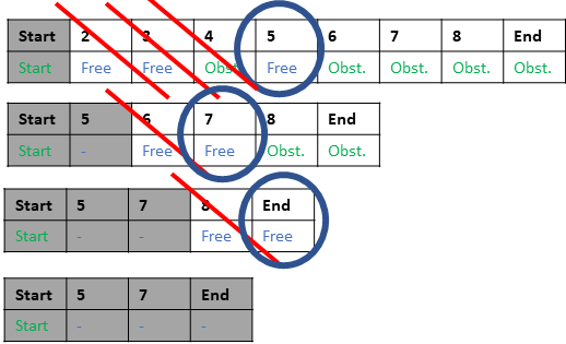
The planned returned from the back tracking algorithm is simplified using the following process: there are two nested iterations over the final path nodes. The algorithm checks whether there are collision-free straight line connections between every pair of nodes in an ordered fashion. First, it checks the starting point with the other points in the list. Then, the feasible connection with the node that has the largest index is kept and the nodes that have indices in-between the first and such node are discarded from the list. The next iteration begins from the node that was used to simplify the path until the last node is reached. The optimization is performed in the total distance traveled. The process is depicted in Figure 2. All possible connections with the right-most shaded gray node are checked. It is visible how the path is simplified.
Algorithm 1: Proposed RRT Algorithm Pseudocode
Input: Start, Goal, Map
Output: RRT_path
Initialize no_iter, edges1 and edges2.
verts1 ← start; verts2 ← goal
flag1 ← False; flag2 ← False

For k = 2 to num_iter:
    While True:
        If (flag1 == false):
            q_sampled1 ← sample_point(map)
        If (flag2 == false):
            q_sampled2 ← sample_point(map)
        point_on_obstacle1 ← collide(map, q_sampled1)
        point_on_obstacle2 ← collide(map, q_sampled2)
        near_index1 ← dsearchn(verts1, q_sampled1)
        near_index2 ← dsearchn(verts2, q_sampled2)
        path_check1 ← [verts1(near_index1), q_sampled1]
        path_check2 ← [verts2(near_index2), q_sampled2]
        path_on_obstacle1 ← path_collision_checker(map, path_check1)
        path_on_obstacle2 ← path_collision_checker(map, path_check2)

        If (point_on_obstacle1 == False) AND (path_on_obstacle1 == False):
            edges1{k-1,1} ← verts1(near_index1,1:3)
            edges1{k-1,2} ← q_sampled1
        If (point_on_obstacle2 == False) AND (path_on_obstacle2 == False):
            edges2{k-1,1} ← verts2(near_index2,1:3)
            edges2{k-1,2} ← q_sampled2
        If (flag1 == True) AND (flag2 == True):
            flag1 = flag2 = false
            final_path_check ← (q_sampled1, q_sampled2)
            path_on_obstacle_final ← path_collision_checker(map, final_path_check)
            If (path_on_obstacle_final == False):
                flag_tree_connected = True
            break

    verts1 ← q_sampled_1; verts2 ← q_sampled_2
    If (flag_tree_connected = True):
        break

If (NOT Converged):
    Return ERROR
RRT_path ← back_tracking(start, goal, edges1, edges2, k-1)
RRT_path ← path_simplification(RRT_path, map)
4. RESULTS
For the sake of this application we have prepared a map of a room, where fire is considered an obstacle. In addition to fire, there are other obstacles that may exist in a house. We assume that every obstacle is convex and is characterized by a polyhedral geometric shape. Non-convex obstacles can be described as a union of convex obstacles.
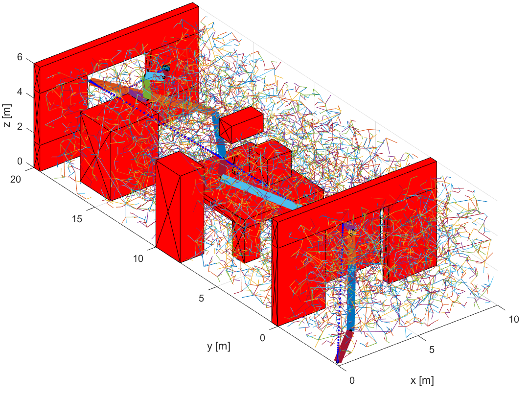
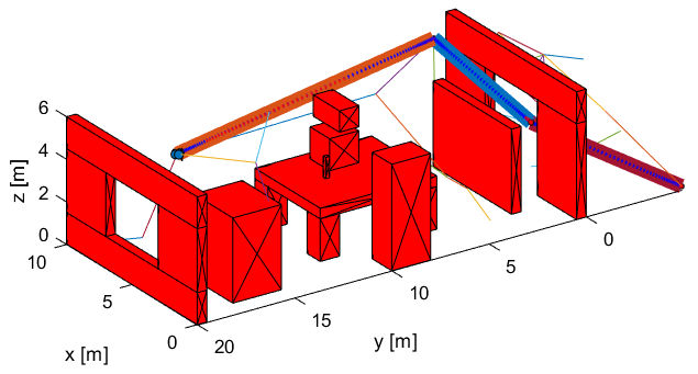
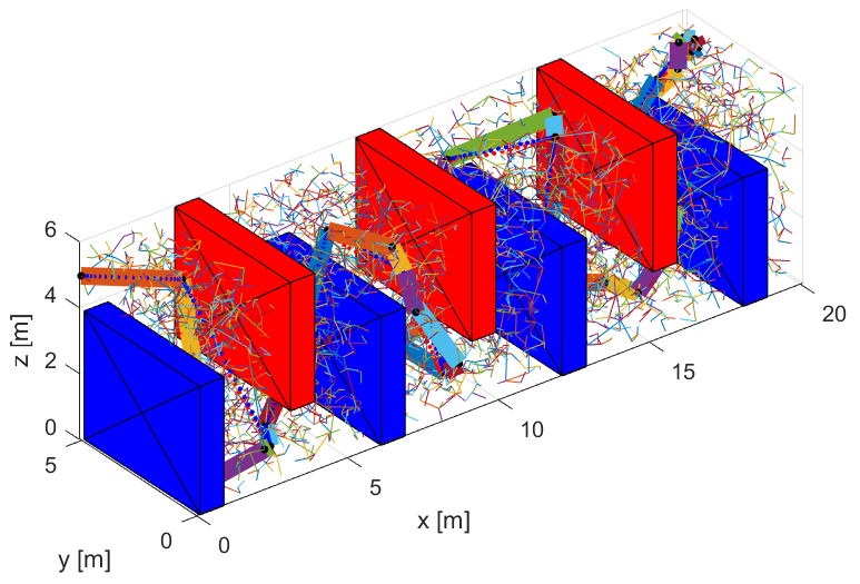
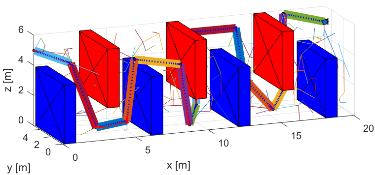
The B-RRT algorithm, Figure 4, is compared to a normal RRT algorithm Figure 3. In Figure 5, another map is provided for both algorithms, which does not necessarily imply that it is a room on fire, but it is added for the sake of comparing both algorithms in a different setup. The obstacles are marked in red and blue, and the connections of the trees can be seen clearly. The final path is shown with thick line segments. The tree grows within the boundaries of the map and those are the the maximum values of the axes. The initial and final position are located more or less on the extremes of the map.
For both algorithms, we performed a number of experimental runs on the Matlab environment and two of the basic criteria, run time and number of iterations are presented in Table 1. The code with which the results had been produced can be found in the attached files. The values provided come as a result of 1000 runs for each algorithm. It needs to be mentioned that all tests were conducted on the same machine, running an Intel 8550U processor. Furthermore a video link can be found on the caption of both figures, with the video of RRT accelerated 500 times, a value that can be derived from how much faster B-RRT runs, in order to be watchable in a lower amount of time.
Table 1: Performance comparison of RRT and B-RRT
| Algorithm name |
run time (sec) |
no. of iterations |
| min |
mean |
max |
min |
mean |
max |
| RRT |
1.5434 |
31.9930 |
124.4538 |
555 |
11124 |
42589 |
| proposed B-RRT |
0.0982 |
1.1913 |
17.4709 |
2 |
55.0983 |
302 |
5. DISCUSSION
From the results, it can be seen that not only the proposed B-RRT algorithm produces a better trajectory, but also converges much faster in a shorter amount of time. If the maximum number of sample iterations is reduced significantly, e.g. 300, the RRT never converges, while the proposed algorithm does it almost every time. Our algorithm reduces the total computational stress significantly due to the lower number of iterations it requires. However, it should be noted that every iteration stresses the computational system more, as two trees are being computed simultaneously, which justifies the maximum time of the proposed B-RRT compared to RRT, even though the last requires much more samples.
A bidirectional algorithm, such as the one proposed, can show significantly better results in a map such as that of Figure 5, where the number of iterations needed to converge to the goal, especially in the region near it, is noticeably smaller. That depends on the tolerance region that is set. The later, is calculated based on difference parameters like the minimum obstacle size considered, etc.
The aforementioned, exploits the advantages of a bidirectional algorithm. However, the proposed algorithm, uses a collision free condition to connect the two trees. This 'heuristic' works most efficiently when we can expect relatively open spaces for the majority of the planning. For example, for a space with no obstacles in between, a connection would be immediate.
The complexity of the algorithm is: 2O(\(|V/2|\) log(\(|V/2|\) + \(|E/2|\))) + O\((V_F^2)\). The first part of the sum refers to the time complexity of bi-directional RRT (B-RRT), and the second part relates to the optimization (or simplification) of the path obtained that has \(V_F\) nodes, which consists of two loops: one that iterates over the nodes and the second one, iterates over the paths connecting the node of the first loop with the others. Therefore, the algorithm optimizes the path obtained in the bi-directional RRT, however, this does not mean it will become globally optimal. The optimization reduces the distance to travel of the path obtained in. Just as conventional RRT, the proposed B-RRT is probabilistically complete because the probability to finding a solution, if one exists, approaches one as the number of samples taken reaches infinity. The B-RRT does not ensure optimality even on the limit, based on the fact that RRT does not ensure either asymptotic optimality[9].
The variant, RRT* performs better since it provides the global optimal path. However, it is not yet clear if the compilation time required for RRT* is greater than that of the proposed method and that can be investigated in the future. For future work, the presented B-RRT method can be improved to B-RRT* so the globally optimal solution can be found if possible. In order to do so, the RRT section needs to be adapted to RRT*.
REFERENCES
- D. Devaurs, T. Siméon and J. Cortés, "Enhancing the Transition-based RRT to Deal with Complex Cost Spaces," IEEE International Conference on Robotics and Automation, 2013.
- S. K. Choudhury, S. Dukkipati, P. Kumar and V. V.S., "A RRT* Motion Planning Approach for the Generalized Multi-Vehicle Heterogeneous PnP Problem," IEEE International Conference on Intelligent Robots and Systems, 2017.
- P. G. Tang, "An Improved RRT*-Based Path Planning Approach for Fixed-Wing UAV," 2020.
- D. A. Reyes Castro, S. Bhattacharya and N. Hover, "Path Planning using Cylindrical Vector Field and Timed Elastic Band for Multi-rotor UAVs in Unknown Environments," Journal of Guidance, Control, and Dynamics, 2019.
- D. Quan, "System Dynamic Modelling and Control," in Introduction to Multicopter Design and Control, Springer, 2020.
- D. S. Sabatino, "Quadrotor Control: Modeling, Nonlinear Control Design, and Simulation," 2015.
- T. Lee, M. Leok and N. McClamroch, "Nonlinear Robust Tracking Control of a Quadrotor UAV on SE(3)," Asian Journal of Control, 2013.
- M. S. Triantafyllou and F. S. Hover, "Maneuvering and Control of Marine Vehicles," 2003.
- I. A. Qureshi and X. Ma, "Improvement and Implementation of the RRT* Algorithm," 2015.
- Apostolides, G. D. Singh, K. Voogd, and M. Gkozntaris. RRT algorithm. TU Delft. [Online]. Available: VIDEO_1
- Apostolides, G. D. Singh, K. Voogd, and M. Gkozntaris. Proposed B-RRT algorithm. TU Delft. [Online] Available: VIDEO_2